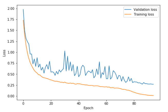
绘制图形的工具比较多,常用的有matplotlib,plotly,以及pytorch的visdom。matplotlib用的比较多,功能也十分强大也比较底层。可以设置的参数也多,用起来比较麻烦。相反visdom使用更加简便,也提供了足够的功能。两者最大的区别是,visdom是运行于云端的,自身也提供了存储,适合简单地分析使用。而matplotlib能绘制更加复杂,个性化的图。因此我打算在项目运行中使用visdom,这样我可以在云端实时监控训练状态。在论文中,如果需要更复杂的图就使用matplotlib。而plotly制作的图形更加强大,也提供云端访问和数据编辑功能,作为企业级的数据展示更加合理。

建议使用半天时间掌握visdom,和几类基本图形。再花半天时间理解matplotlib的概念和用法,毕竟很多代码是使用这个的且与matlab类似,要能读懂。编写项目展示的时候使用plotly,这个比较专业,最好是团队中有专人掌握,一般没必要精通。

visdom

基本概念: window,env,state,filter,view

env->window - view

window

window是承载内容的主体,其数据存储在state中(.visdom目录下会创建json文件)。他是一个UI组件,可以显示plots, images, and text。还可以注册callback来监听用户的操作。

environment

所有windowy以env为一组进行组织。

当有大量数据需要实时绘制时。如果需要对比他们,最好放在同一个env下。多个env会消耗大量资源

filter

filter使用正则表达式来匹配window的title。

view

view是window的排列方式

使用

  1. Visdom实例
    visdom Arguments

    • server
    • port
    • offline 启用时将数据存在本地
    • log_to_filename
  2. 绘图

    • vis.image : CxHxW,显示一张图片。但是可以存储一组store_history
    • vis.images : B x C x H x W
    • vis.text : 可以嵌入 HTML
    • vis.properties : 输入组件,Callback
    • vis.audio : audio
    • vis.video : videos
    • vis.svg : SVG object
    • vis.matplot : matplotlib plot
  3. Plotly
    使用plotly提供常用数据的可视化,推荐使用这种方式。这种方式存储数据,而不是图像。

    • vis.scatter : 2D or 3D scatter plots
    • vis.line : line plots
    • vis.stem : stem plots
    • vis.heatmap : heatmap plots
    • vis.bar : bar graphs
    • vis.histogram : histograms
    • vis.boxplot : boxplots
    • vis.surf : surface plots
    • vis.contour : contour plots
    • vis.quiver : quiver plots
    • vis.mesh : mesh plots
      demo
      扩展,可以传入一个字典结构opts
    • opts.title : figure title
    • opts.width : figure width
    • opts.height : figure height
    • opts.showlegend : show legend (true or false)
    • opts.xtype : type of x-axis (‘linear’ or ‘log’)
    • opts.xlabel : label of x-axis
    • opts.xtick : show ticks on x-axis (boolean)
    • opts.xtickmin : first tick on x-axis (number)
    • opts.xtickmax : last tick on x-axis (number)
    • opts.xtickvals : locations of ticks on x-axis (table of numbers)
    • opts.xticklabels : ticks labels on x-axis (table of strings)
    • opts.xtickstep : distances between ticks on x-axis (number)
    • opts.xtickfont : font for x-axis labels (dict of font information)
    • opts.ytype : type of y-axis (‘linear’ or ‘log’)
    • opts.ylabel : label of y-axis
    • opts.ytick : show ticks on y-axis (boolean)
    • opts.ytickmin : first tick on y-axis (number)
    • opts.ytickmax : last tick on y-axis (number)
    • opts.ytickvals : locations of ticks on y-axis (table of numbers)
    • opts.yticklabels : ticks labels on y-axis (table of strings)
    • opts.ytickstep : distances between ticks on y-axis (number)
    • opts.ytickfont : font for y-axis labels (dict of font information)
    • opts.marginleft : left margin (in pixels)
    • opts.marginright : right margin (in pixels)
    • opts.margintop : top margin (in pixels)
    • opts.marginbottom: bottom margin (in pixels)
      自定义绘图 将数据和参数传入Plotly

      1
      2
      3
      4
      5
      6
      7
      8
      9
      import visdom
      vis = visdom.Visdom()

      trace = dict(x=[1, 2, 3], y=[4, 5, 6], mode="markers+lines", type='custom',
      marker={'color': 'red', 'symbol': 104, 'size': "10"},
      text=["one", "two", "three"], name='1st Trace')
      layout = dict(title="First Plot", xaxis={'title': 'x1'}, yaxis={'title': 'x2'})

      vis._send({'data': [trace], 'layout': layout, 'win': 'mywin'})

      注意data中必须添加type='custom'才能生效。而且一些内容无法显示。如果有大量内容需要使用这个功能,不如直接使用plotly。

  4. demo

matplotlib

基本概念

figure表示一张图,Axes表示一个绘图元素,一个figure可以包含多个axes。axis表示轴,可以设置刻度,标签,范围等。
在内部matplotlib有一个状态机来存储当前的figure与axes,默认情况下plot会自动创建一个新的或者重复使用上一个axes。subplot 在当前figure下创建多个axes.subplots创建新的figure和axes。

Call signatures::

  subplot(nrows, ncols, index, **kwargs)
  subplot(pos, **kwargs)
  subplot(ax)

而且subplot(3,2,1)等价于subplot(321),其中index选中的axes可以用plt.plot来绘图。也可以用返回值fig,ax=subplot(321)来绘图。

交互模式

1
2
3
4
5
import matplotlib.pyplot as plt
plt.ion()
plt.plot([1.6, 2.7]) #立即显示
plt.ioff()
plt.show() # 手动显示

plotly

这篇文章很不错,介绍了plotly的offline,graph,trace,layout
进阶需要参考官方文档

原文
本文介绍一种能够快速获得模型结果,并提高精度。首先介绍Leslie Smith在超参数(hyper-parameters )方面的工作。他将其称为1cycle policy,能够快速地训练复杂模型。

大学习率


0-41个epoch中,learning rate从0.08线性增长到0.8,然后在42-82个epoch内从0.8回落到0.08.
high learning rate可以起到regularization的效果防止过拟合。这相当于防止跨入一个小的局部最优解。这表明SGD在寻找一个宽阔平坦的区域

Supplements

1cycle policy
Super-Convergence
Deep Residual Learning for Image Recognition

Copies and Views

视图共享数据,但不是同一个对象。而复制会重新分配内存,在实际中应该尽量避免复制操作。

1
2
a = np.arange(12)
b = a # no new object is created

b与a是完全等价的

View or Shallow Copy

也可以称作浅拷贝,它创建了新的对象,但是使用了相同的数据。

1
2
3
4
5
6
7
8
9
10
11
12
13
14
15
16
17
>>> a = np.arange(12)
>>> c = a.view()
>>> c is a
False
>>> c.base is a # c is a view of the data owned by a
True
>>> c.flags.owndata
False
>>>
>>> c.shape = 2,6 # a's shape doesn't change
>>> a.shape
(3, 4)
>>> c[0,4] = 1234 # a's data changes
>>> a
array([[ 0, 1, 2, 3],
[1234, 5, 6, 7],
[ 8, 9, 10, 11]])

Slicing an array returns a view of it:

1
2
3
4
5
6
7
8
9
10
11
12
13
14
15
16
17
18
19
>>> s = a[ : , 1:3]     # spaces added for clarity; could also be written "s = a[:,1:3]"
>>> s[:] = 10 # s[:] is a view of s. Note the difference between s=10 and s[:]=10
>>> a
array([[ 0, 10, 10, 3],
[1234, 10, 10, 7],
[ 8, 10, 10, 11]])
Deep Copy
The copy method makes a complete copy of the array and its data.

>>> d = a.copy() # a new array object with new data is created
>>> d is a
False
>>> d.base is a # d doesn't share anything with a
False
>>> d[0,0] = 9999
>>> a
array([[ 0, 10, 10, 3],
[1234, 10, 10, 7],
[ 8, 10, 10, 11]])

Deep Copy

完全复制数据。耗时大。

1
2
3
4
5
6
7
8
9
10
>>> d = a.copy()                          # a new array object with new data is created
>>> d is a
False
>>> d.base is a # d doesn't share anything with a
False
>>> d[0,0] = 9999
>>> a
array([[ 0, 10, 10, 3],
[1234, 10, 10, 7],
[ 8, 10, 10, 11]])

判断是否发生了拷贝

a.__array_interface__['data']返回数据指针 , a.flags.owndata 是否拥有数据, a.base is b.base 检测父元素。经过测试,第三种方法最为有效。

1
2
3
4
5
a= np.arange(36).reshape(6,6) #第二种方法失效,reshape返回一个view。
b= a[1,:] # 第一种方法失效
c=a[::2,::3]
d = c.reshape(2,3)
d.base is a.base # False, 由于c在空间上不连续,导致reshape重新开辟一块空间。

选择合适的操作

选择

以下方式操作的都是view

1
2
a[1:2, 3:6]    # 切片 slice
a[::2] # 跳步

而下面会导致copy

1
2
3
a_copy1 = a[[1,4,6], [2,4,6]]   # 用 index 选
a_copy2 = a[[True, True], [False, True]] # 用 mask
a_copy4 = a[a[1,:] != 0, :] # fancy indexing

np中提供了np.take(),np.compress方法,功能与上面类似,但是更加高效。

变形

numpy 提供了几种方法:a.reshape(),a.shape=(),a.resize(),a.flatten(),a.ravel().
其中a.shape=() 必返回视图。
a.flatten()必返回一个拷贝,如果不是必要应该避免。
而其他操作在有需要的时候复制。

赋值

就地操作 a+=2
一些方法带有out参数,可以直接将结果写入out变量从而避免copy。

1
np.add(a, 1, out=a)    # 0.008843

复制元素

np.stride_tricks.as_strided
这个方法可以起到分块的作用,同时也能改变矩阵的形状,大小,但是它返回的其实是一个view,因此十分高效。
首先把A看作是一维的,然后给出想要的形状,最后规定每一步的长度。

比如im2col算法就有一个简单高效的实现:

1
2
3
4
5
6
7
8
9
10
11
def im2col_3d(A, BSZ: tuple):
# Parameters
channel, r, c = A.shape
s0, s1, s2 = A.strides
nrows = r - BSZ[0] + 1
ncols = c - BSZ[1] + 1
shp = channel, BSZ[0], BSZ[1], nrows, ncols
strd = s0, s1, s2, s1, s2

out_view = np.lib.stride_tricks.as_strided(A, shape=shp, strides=strd)
return out_view.reshape( channel * BSZ[0] * BSZ[1], -1)

Trick

前面提到如果数组在内存空间中不连续,那么在一些操作就无法在原来的地方进行。如reshape。但是np视乎做过一些优化,如果在切片的步长是一个整数,那么就可以将其看作是连续的。

1
2
3
4
5
6
7
8
a= np.arange(72).reshape(12,6) 
c=a[::2,::3]
c.shape=12 #出错
e=a.ravel()[::3]
f1=e[::4]
f2=e[1::4]
f1.shape=2,3
f1.base is a.base # True

那么对其进行2次定长切片处理就能得到我们想要的东西。

疑问

1
2
3
4
5
6
7
8
9
10
11
12
13
14
15
16
17
18
19
20
21
22
23
24
25
26
27
28
29
30
31
32
33
34
35
36
37
38
39
40
41
42
43
44
45
46
47
48
49
50
51
52
53
54
55
56
57
58
59
60
img = np.random.random((100, 3, 32, 32))
w = np.random.random((3, 5, 5))


def im2col_4d(A, BSZ: tuple):
# Parameters
m, channel, r, c = A.shape
s0, s1, s2, s3 = A.strides
nrows = r - BSZ[0] + 1
ncols = c - BSZ[1] + 1
shp = m, channel, BSZ[0], BSZ[1], nrows, ncols
strd = s0, s1, s2, s3, s2, s3
out_view = np.lib.stride_tricks.as_strided(A, shape=shp, strides=strd)
return out_view.reshape(m, channel * BSZ[0] * BSZ[1], -1)


def im2col_3d(A, BSZ: tuple):
# Parameters
channel, r, c = A.shape
s0, s1, s2 = A.strides
nrows = r - BSZ[0] + 1
ncols = c - BSZ[1] + 1
shp = channel, BSZ[0], BSZ[1], nrows, ncols
strd = s0, s1, s2, s1, s2

out_view = np.lib.stride_tricks.as_strided(A, shape=shp, strides=strd)
return out_view.reshape( channel * BSZ[0] * BSZ[1], -1)

def c1():

value = np.zeros((100, 28, 28))
for i in range(100):
for c in range(3):
# 转列 88ms
col = im2col_sliding_strided(img[i, c, ...], (5, 5))
# dot 用时30ms
value[i, ...] += w[c].ravel().dot(col).reshape(28, 28)
return value


def c2():
# 高维数组的乘法效率很低,这个方法反而是最慢的
# 355ms 这个方法也变慢了我感觉很意外
col = im2col_4d(img, (5, 5))
# dot 用时150ms
return w.ravel().dot(col).reshape(-1, 28, 28)

def c3():
# 使col仍为二维,效率最高
value = np.zeros((100, 28, 28))
for i in range(100):
# 66 ms
col = im2col_3d(img[i, ...], (5, 5))
# 20ms
value[i, ...] = w.ravel().dot(col).reshape(28, 28)
return value

print(use_time(c1,10))
print(use_time(c2,10))
print(use_time(c3,10))

以上代码实现卷积运算时发现将所有数据统一处理反而是最慢的。结果表明c3,每次处理一组数据是最快的。其中大数组的reshape慢于多个小数组的reshape,同样点积也是大的慢。

##

Refences

为什么用 Numpy 还是慢, 你用对了吗?
Tutorial
高效分块操作